Python: Divvy Bike Share Insights

Overview

The goal of this project is to look at bike ride data for insights and trends from Divvy, a bike share company based out of Chicago. The data was downloaded from https://divvy-tripdata.s3.amazonaws.com/index.html. The data is compressed in .zip format and is separated by month. Each zip file contains a .csv file that contains individaul bike rides, subcription type, timestamps and start and end locations.

Technologies and Software

Python: I will use Python to unzip files and create a comprehensive single csv file.
Pandas: I will use the Pandas package within Python to make a dataframe of the data and make aggregrations dataframes.
Matplotlib: I will use the Matplotlib package within Python to make visualizatons of data in order to easily see trends.

Questions to Answer

What are the count of rides by subscription per month?
What are the peak periods of rides?
What are the average ride times by subscription?
What are the most popular start locations?

Steps

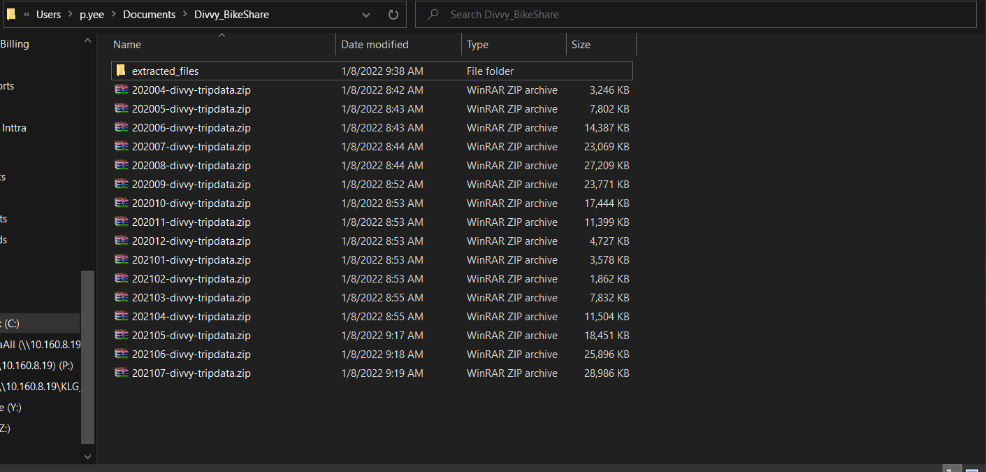
1. Download all the Zip files to localc computer

I have downloaded all the files to my local directory: C:\Users\p.yee\Documents\Divvy_BikeShare\zip_files

2. Create a Python script to unzip files in directory

I have used the following script:


from zipfile import ZipFile
import os

home_dir = r"C:\Users\p.yee\Documents\Divvy_BikeShare"
zip_source = home_dir+ "\\zip_files\\"
zip_target = home_dir+r"\extracted_files"
file_list = os.listdir(zip_source)

for file_name in file_list:
    print(file_name)
    with ZipFile(zip_source + file_name, 'r') as zipObj:
        # Get a list of all archived file names from the zip
        listOfFileNames = zipObj.namelist()
        # Iterate over the file names
        for csv_file in listOfFileNames:
            # Check filename endswith csv
            if csv_file.endswith('.csv'):
                # Extract a single file from zip
                zipObj.extract(csv_file, zip_target)

Files will be unizziped here:

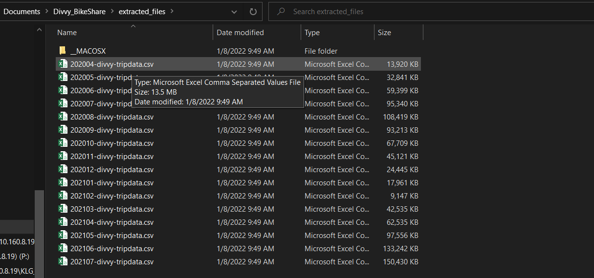
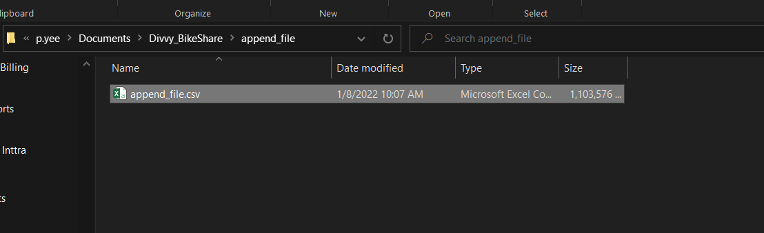
3. Create a script to append all the csv files to a single csv file

It will be easier to do the analysis on a single dataset. Also knowing the dataset has the same headers and format it makes sense to append this data. Use the following:


import os
import pandas as pd

home_dir = r"C:\Users\p.yee\Documents\Divvy_BikeShare"
zip_target = home_dir+r"\extracted_files"
append_target =home_dir+ r"\append_file"


all_files=os.listdir(zip_target)

append_file = pd.DataFrame()

for file_name in all_files:
	if file_name.endswith(".csv"):
		df=pd.read_csv(zip_target +"\\" + file_name)
		append_file=pd.concat([append_file, df])

append_file.to_csv(append_target + "\\" + "append_file.csv",index=False)

All Files will be appeneded to a single file here:

4. Create a script that will aggregrate the data and present data visualizations

I have used the following script:


# questions to answer
# 1. What are the count of rides by subscription per month?
# 2.  What are the peak periods of rides?
# 3. What are the average ride times by subscription?
# 4.  What are the most popular start points?


import pandas as pd
import matplotlib.pyplot as plt


home_dir = r"C:\Users\p.yee\Documents\Divvy_BikeShare"
append_target =home_dir+r"\append_file"





append_df = pd.read_csv(append_target + "\\" + "append_file.csv")

#clean nulls
#nan_df = append_df[append_df.isna().any(axis=1)]
#print(nan_df.head())
#covert data types

# remove nan values, replace with 0
append_df['start_station_id']=pd.to_numeric(append_df['start_station_id'], errors='coerce').fillna(0)
append_df['end_station_id']=pd.to_numeric(append_df['end_station_id'], errors='coerce').fillna(0)

# convert to int
append_df['start_station_id'] = append_df['start_station_id'].astype('int32')
append_df['end_station_id'] = append_df['end_station_id'].astype('int32')

# convert to datetime
append_df['started_at'] = append_df['started_at'].astype('datetime64')
append_df['ended_at'] = append_df['ended_at'].astype('datetime64')

#add columns
append_df['ride_time'] = (append_df['ended_at'] - append_df['started_at']).astype('timedelta64[m]')
append_df['month_year'] = pd.to_datetime(append_df['started_at']).dt.to_period('M')
append_df['hour_ride'] = append_df['started_at'].dt.hour

# What are the count of rides by subscription per month?
total_count_df = append_df.groupby(['month_year','member_casual'], as_index=False)['ride_id'].count()


plt.figure('1')
casual_count = total_count_df.loc[total_count_df['member_casual'] == 'casual']

member_count = total_count_df.loc[total_count_df['member_casual'] == 'member']

#matplotlib cant plot datetime on x axis so convert to string
casual_count['month_year'] = casual_count['month_year'].astype('str')
member_count['month_year'] = member_count['month_year'].astype('str')




plt.plot(casual_count['month_year'],casual_count['ride_id'],label ='Casual Rider')
plt.plot(member_count['month_year'],member_count['ride_id'],label ='Member Rider')

plt.xlabel('Year Month')
plt.ylabel('Count of Rides')
plt.title('Rides by Month Year by Subscription')
plt.legend()
plt.xticks(rotation = 45)
plt.tight_layout()
plt.savefig(r'C:\Users\p.yee\Documents\Divvy_BikeShare\figures\Rides_Month_Count.png')


# 2. What are the average ridetimes by subscription?
plt.figure('2')
avg_ride_time = append_df.groupby(['member_casual'], as_index=False)['ride_time'].mean()



plt.bar(avg_ride_time['member_casual'],avg_ride_time['ride_time'])
plt.xlabel('Subscription Type')
plt.ylabel('Average Ride Time in Minutes')


plt.title('Average Ride Time by Subscription')
plt.tight_layout()
plt.savefig(r'C:\Users\p.yee\Documents\Divvy_BikeShare\figures\Average_Ride_Time.png')


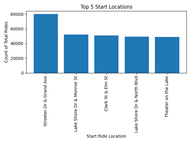
plt.figure(3)
N = 5
#top_N = append_df.groupby(["start_station_name"])['ride_id'].sum().sort_values(ascending=False).head(N)
top_n_station = append_df.groupby(['start_station_name'], as_index=False)['ride_id'].count().sort_values(by='ride_id', ascending=False).head(N)


plt.bar(top_n_station['start_station_name'],top_n_station['ride_id'])
plt.xlabel('Start Ride Location')
plt.xticks(rotation = 90)
plt.ylabel('Count of Total Rides')


plt.title(f'Top {N} Start Locations')
plt.tight_layout()
plt.savefig(r'C:\Users\p.yee\Documents\Divvy_BikeShare\figures\Top_Start_Locations.png')


#   What are the peak periods of rides?
plt.figure(4)
peak_periods = append_df.groupby(['hour_ride'], as_index=False)['ride_id'].count()
plt.plot(peak_periods['hour_ride'],peak_periods['ride_id'])
plt.xlabel('Hour')
plt.ylabel('Count of Rides')
plt.title('Peak Ride Times by Hour')
plt.tight_layout()
plt.savefig(r'C:\Users\p.yee\Documents\Divvy_BikeShare\figures\Peak_Times.png')

Results

Lets review the questions:

What are the count of rides by subscription per month?

You can see from the following line chart created by Matplotlib that the peak seasons for bike sharing is in late spring to late autumn. This makes sense because Chicago is in the northern part of the US and it is not very practical to ride a bicycle in the winter. In terms of historic data the 'casual' subscription biker has exceeded the 'member' subscription biker until May of 2021. It will be interesting to see what promotional tactics were used by Divvy in order to change bikers from 'casuals' to 'members'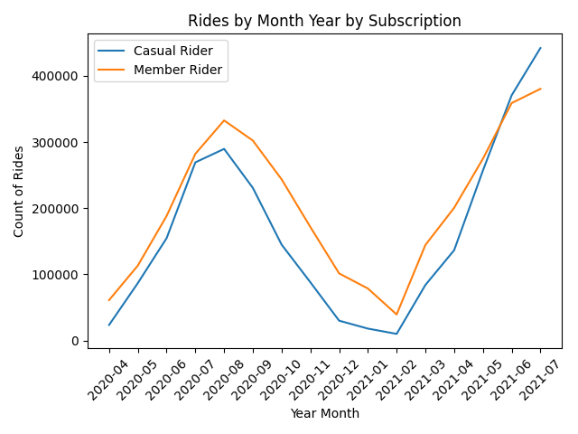

What are the peak periods of rides?

You can see the peak time rises between 10:00 am and 05:00 pm. From this Divvy can see what are low times where they can move unused bikes to more popular locations.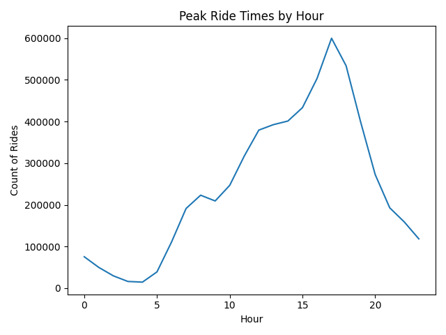

What are the average ride times by subscription?

You can see that the casual rider time is more than double than the member rider time. From this we can see that perhaps the casual rider is not aware of the benefits of membership and the potential cost savings.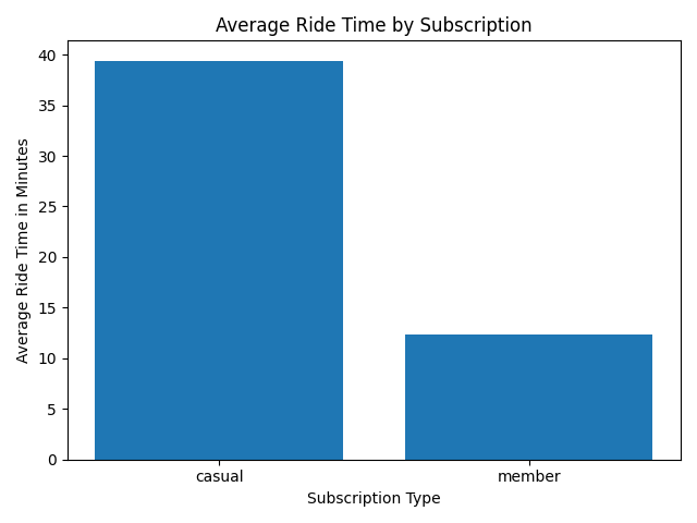

What are the most popular start locations?

From this we can see the top locations. It is important to keep these locations fully stocked.

Patrick Yee

Divvy Bike Share: Data Cleaning and Visualization using Python